Reshaping data with `tidyr`

Practical Computing and Data Science Tools

Annoucements

Midterm II is Thursday, November 14th.
Material on the midterm will include all material through Week 11.

Agenda

Continuation and review of combining tibbles (i.e. data joins)
Reshaping data with tidyr

Data Joins

Data Joins in `R`

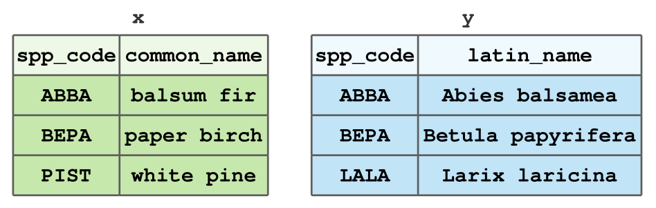
Recall the x and y tibbles from last time.

Types of Data Joins

The dplyr package includes functions for two general types of joins:

Mutating joins, which combine the columns of tibbles x and y, and
Filtering joins, which match the rows of tibbles x and y.

Think of how mutate() adds columns to a tibble, while filter() removes rows.

Mutating Joins

dplyr contains four mutating joins:

left_join(x, y) keeps all rows of x, but if a row in y does not match to x, an NA is assigned to that row in the new columns.
right_join(x, y) is equivalent to left_join(y, x), except for column order.
inner_join(x, y) keeps only the rows matched between x and y.
full_join(x, y) keeps all rows of both x and y.

Filtering Joins

dplyr contains two filtering joins:

semi_join(x, y) keeps all the rows in x that have a match in y.
anti_join(x, y) removes all the rows in x that have a match in y.

Note: Unlike mutating joins, filtering joins do not add any columns to the data.

Loading data

We’ll create the x and y tibbles in R:

library(tidyverse)
x <- tibble(spp_code = c("ABBA", "BEPA", "PIST"),
            common_name = c("balsum fir", "paper birch", "white pine"))

y <- tibble(spp_code = c("ABBA", "BEPA", "LALA"),
            latin_name = c("Abies balsamea", 
                           "Betula papyrifera",
                           "Larix laricina"))

Loading data

We’ll create the x and y tibbles in R:

# A tibble: 3 × 2
  spp_code common_name
  <chr>    <chr>      
1 ABBA     balsum fir 
2 BEPA     paper birch
3 PIST     white pine

# A tibble: 3 × 2
  spp_code latin_name       
  <chr>    <chr>            
1 ABBA     Abies balsamea   
2 BEPA     Betula papyrifera
3 LALA     Larix laricina

Q1. Write the code to get this output

# A tibble: 3 × 3
  spp_code common_name latin_name       
  <chr>    <chr>       <chr>            
1 ABBA     balsum fir  Abies balsamea   
2 BEPA     paper birch Betula papyrifera
3 PIST     white pine  <NA>

01:00

Q1. Write the code to get this output

left_join(x, y, by = "spp_code")

# A tibble: 3 × 3
  spp_code common_name latin_name       
  <chr>    <chr>       <chr>            
1 ABBA     balsum fir  Abies balsamea   
2 BEPA     paper birch Betula papyrifera
3 PIST     white pine  <NA>

Q2. Write the code to get this output

# A tibble: 4 × 3
  spp_code common_name latin_name       
  <chr>    <chr>       <chr>            
1 ABBA     balsum fir  Abies balsamea   
2 BEPA     paper birch Betula papyrifera
3 PIST     white pine  <NA>             
4 LALA     <NA>        Larix laricina

01:00

Q2. Write the code to get this output

full_join(x, y, by = "spp_code")

# A tibble: 4 × 3
  spp_code common_name latin_name       
  <chr>    <chr>       <chr>            
1 ABBA     balsum fir  Abies balsamea   
2 BEPA     paper birch Betula papyrifera
3 PIST     white pine  <NA>             
4 LALA     <NA>        Larix laricina

Q3. Write the code to get this output

# A tibble: 3 × 3
  spp_code latin_name        common_name
  <chr>    <chr>             <chr>      
1 ABBA     Abies balsamea    balsum fir 
2 BEPA     Betula papyrifera paper birch
3 LALA     Larix laricina    <NA>

01:00

Q3. Write the code to get this output

left_join(y, x, by = "spp_code")

# A tibble: 3 × 3
  spp_code latin_name        common_name
  <chr>    <chr>             <chr>      
1 ABBA     Abies balsamea    balsum fir 
2 BEPA     Betula papyrifera paper birch
3 LALA     Larix laricina    <NA>

Q4. Write the code to get this output

# A tibble: 3 × 3
  spp_code common_name latin_name       
  <chr>    <chr>       <chr>            
1 ABBA     balsum fir  Abies balsamea   
2 BEPA     paper birch Betula papyrifera
3 LALA     <NA>        Larix laricina

01:00

Q4. Write the code to get this output

right_join(x, y, by = "spp_code")

# A tibble: 3 × 3
  spp_code common_name latin_name       
  <chr>    <chr>       <chr>            
1 ABBA     balsum fir  Abies balsamea   
2 BEPA     paper birch Betula papyrifera
3 LALA     <NA>        Larix laricina

Q5. Write the code to get this output

# A tibble: 2 × 3
  spp_code common_name latin_name       
  <chr>    <chr>       <chr>            
1 ABBA     balsum fir  Abies balsamea   
2 BEPA     paper birch Betula papyrifera

01:00

Q5. Write the code to get this output

inner_join(x, y, by = "spp_code")

# A tibble: 2 × 3
  spp_code common_name latin_name       
  <chr>    <chr>       <chr>            
1 ABBA     balsum fir  Abies balsamea   
2 BEPA     paper birch Betula papyrifera

Q6. Write the code to get this output

# A tibble: 4 × 3
  spp_code latin_name        common_name
  <chr>    <chr>             <chr>      
1 ABBA     Abies balsamea    balsum fir 
2 BEPA     Betula papyrifera paper birch
3 LALA     Larix laricina    <NA>       
4 PIST     <NA>              white pine

01:00

Q6. Write the code to get this output

full_join(y, x, by = "spp_code")

# A tibble: 4 × 3
  spp_code latin_name        common_name
  <chr>    <chr>             <chr>      
1 ABBA     Abies balsamea    balsum fir 
2 BEPA     Betula papyrifera paper birch
3 LALA     Larix laricina    <NA>       
4 PIST     <NA>              white pine

Consider a third tibble, `z`:

z <- x %>%
  rename(species_code = spp_code)
z

# A tibble: 3 × 2
  species_code common_name
  <chr>        <chr>      
1 ABBA         balsum fir 
2 BEPA         paper birch
3 PIST         white pine

Q7. Write the code to get this output

# A tibble: 3 × 3
  species_code common_name latin_name       
  <chr>        <chr>       <chr>            
1 ABBA         balsum fir  Abies balsamea   
2 BEPA         paper birch Betula papyrifera
3 PIST         white pine  <NA>

01:00

Q7. Write the code to get this output

left_join(z, y, by = c("species_code" = "spp_code"))

# A tibble: 3 × 3
  species_code common_name latin_name       
  <chr>        <chr>       <chr>            
1 ABBA         balsum fir  Abies balsamea   
2 BEPA         paper birch Betula papyrifera
3 PIST         white pine  <NA>

Q8. Write the code to get this output (hint: use a filtering join)

# A tibble: 2 × 2
  spp_code latin_name       
  <chr>    <chr>            
1 ABBA     Abies balsamea   
2 BEPA     Betula papyrifera

01:00

Q8. Write the code to get this output (hint: use a filtering join)

semi_join(y, x, by = "spp_code")

# A tibble: 2 × 2
  spp_code latin_name       
  <chr>    <chr>            
1 ABBA     Abies balsamea   
2 BEPA     Betula papyrifera

Q9. Write the code to get this output (hint: use a filtering join)

# A tibble: 1 × 2
  species_code common_name
  <chr>        <chr>      
1 PIST         white pine

01:00

Q9. Write the code to get this output (hint: use a filtering join)

anti_join(z, y, by = c("species_code" = "spp_code"))

# A tibble: 1 × 2
  species_code common_name
  <chr>        <chr>      
1 PIST         white pine

Q10. Write the code to get this output (hint: use a filtering join)

# A tibble: 1 × 2
  spp_code latin_name    
  <chr>    <chr>         
1 LALA     Larix laricina

01:00

Q10. Write the code to get this output (hint: use a filtering join)

anti_join(y, x, by = "spp_code")

# A tibble: 1 × 2
  spp_code latin_name    
  <chr>    <chr>         
1 LALA     Larix laricina

# or 
anti_join(y, z, by = c("spp_code" = "species_code"))

# A tibble: 1 × 2
  spp_code latin_name    
  <chr>    <chr>         
1 LALA     Larix laricina

Reshaping Data

The `tidyr` package

The tidyr package allows us to transform data from long to wide formats, and back.
A key use of the tidyr package is getting data in tidy format.
But what is tidy format?

Tidy data

“Tidy data” or “tidy format” is a formal concept of how we organize data for analyses, in particular, with tidy data:

Each row of the data correspond to a single observation, and
Each column of the data correspond to a variable.

Tidy data

“Tidy data” or “tidy format” is a formal concept of how we organize data for analyses, in particular, with tidy data:

Each row of the data correspond to a single observation, and
Each column of the data correspond to a variable.

Let’s take a look at a blog post from Julie Lowndes and Allison Horst about tidy data

Tidying data with `tidyr`

Consider the face dataset from IFDAR:

face <- read_csv("../labs/datasets/FACE/FACE_aspen_core_growth.csv") %>%
  select(Rep, Treat, Clone, ID = `ID #`,
        contains(as.character(2001:2005)) & contains("Height"))
face

# A tibble: 1,991 × 9
     Rep Treat Clone    ID `2001_Height` `2002_Height` `2003_Height`
   <dbl> <dbl> <dbl> <dbl>         <dbl>         <dbl>         <dbl>
 1     1     1     8    45            NA            NA            NA
 2     1     1   216    44           547           622           715
 3     1     1     8    43           273           275           305
 4     1     1   216    42           526           619           720
 5     1     1   216    54           328           341           364
 6     1     1   271    55           543           590           634
 7     1     1   271    56           450           502           587
 8     1     1     8    57           217           227           256
 9     1     1   259    58           158           155            NA
10     1     1   271    59           230           241           260
# ℹ 1,981 more rows
# ℹ 2 more variables: `2004_Height` <dbl>, `2005_Height` <dbl>

Tidying data with `tidyr`

Is this data tidy? If so, what does a row represent? What does a column represent?

face

# A tibble: 1,991 × 9
     Rep Treat Clone    ID `2001_Height` `2002_Height` `2003_Height`
   <dbl> <dbl> <dbl> <dbl>         <dbl>         <dbl>         <dbl>
 1     1     1     8    45            NA            NA            NA
 2     1     1   216    44           547           622           715
 3     1     1     8    43           273           275           305
 4     1     1   216    42           526           619           720
 5     1     1   216    54           328           341           364
 6     1     1   271    55           543           590           634
 7     1     1   271    56           450           502           587
 8     1     1     8    57           217           227           256
 9     1     1   259    58           158           155            NA
10     1     1   271    59           230           241           260
# ℹ 1,981 more rows
# ℹ 2 more variables: `2004_Height` <dbl>, `2005_Height` <dbl>

How do we make this data tidy? 🤔

face

# A tibble: 1,991 × 9
     Rep Treat Clone    ID `2001_Height` `2002_Height` `2003_Height`
   <dbl> <dbl> <dbl> <dbl>         <dbl>         <dbl>         <dbl>
 1     1     1     8    45            NA            NA            NA
 2     1     1   216    44           547           622           715
 3     1     1     8    43           273           275           305
 4     1     1   216    42           526           619           720
 5     1     1   216    54           328           341           364
 6     1     1   271    55           543           590           634
 7     1     1   271    56           450           502           587
 8     1     1     8    57           217           227           256
 9     1     1   259    58           158           155            NA
10     1     1   271    59           230           241           260
# ℹ 1,981 more rows
# ℹ 2 more variables: `2004_Height` <dbl>, `2005_Height` <dbl>

Each row should represent a measurement for a given rep, treatment, clone, and ID. But currently, we have multiple measurements on the same row.
Further, we have multiple columns for the “height” variable.
Not tidy!

We need to pivot the data into a longer format!

Enter, pivot_longer().

pivot_longer(), a function from tidyr takes four key arguments:

.data: the data (tibble) you’d like to pivot,
cols: the columns you’d like to pivot,
names_to: the new column that will be created which takes the column names from cols as values, and
values_to: the new column that will be created which takes the column values from cols as values.

Why the long `face`?

face_long <- face %>%
  pivot_longer(
    cols = c("2001_Height", "2002_Height", "2003_Height", 
             "2004_Height", "2005_Height"),
    names_to = "Year_Type",
    values_to = "Height_cm")

Why the long `face`?

face_long <- face %>%
  pivot_longer(
    cols = c("2001_Height", "2002_Height", "2003_Height", 
             "2004_Height", "2005_Height"),
    names_to = "Year_Type",
    values_to = "Height_cm")

Why the long `face`?

face_long <- face %>%
  pivot_longer(
    cols = contains("Height"),
    names_to = "Year_Type",
    values_to = "Height_cm")

A cleaner way to select these columns is to use dplyr’s contains() function.

Why the long `face`?

face_long

# A tibble: 9,955 × 6
     Rep Treat Clone    ID Year_Type   Height_cm
   <dbl> <dbl> <dbl> <dbl> <chr>           <dbl>
 1     1     1     8    45 2001_Height        NA
 2     1     1     8    45 2002_Height        NA
 3     1     1     8    45 2003_Height        NA
 4     1     1     8    45 2004_Height        NA
 5     1     1     8    45 2005_Height        NA
 6     1     1   216    44 2001_Height       547
 7     1     1   216    44 2002_Height       622
 8     1     1   216    44 2003_Height       715
 9     1     1   216    44 2004_Height       716
10     1     1   216    44 2005_Height       817
# ℹ 9,945 more rows

To get tidy data!

Going (back) to wide data

Sometimes, we need to “widen” a dataset to get it into tidy format.
For this example, we will just widen the face_long dataset back to its original form.
tidyr has an aptly named function, pivot_wider().
Key arguments of pivot_wider():
- .data: the tibble to widen,
- names_from: the column that contains values which will be assigned as the new column names,
- values_from: the column that contains

Pivoting wider

face_wide <- face_long %>%
  pivot_wider(names_from = "Year_Type", values_from = "Height_cm")

all_equal(face, face_wide)

[1] TRUE

This results in the same tibble that we started with!

Other useful `tidyr` functions

unite() for pasteing column values together with specified seperators,
The separate_wider_*() family: for splitting columns into multiple new columns:
- separate_wider_delim(): separate by delimiter
- separate_wider_position(): separate by position
- separate_wider_regex(): separate by regular expression

`unite()`: examples

face_long

# A tibble: 9,955 × 6
     Rep Treat Clone    ID Year_Type   Height_cm
   <dbl> <dbl> <dbl> <dbl> <chr>           <dbl>
 1     1     1     8    45 2001_Height        NA
 2     1     1     8    45 2002_Height        NA
 3     1     1     8    45 2003_Height        NA
 4     1     1     8    45 2004_Height        NA
 5     1     1     8    45 2005_Height        NA
 6     1     1   216    44 2001_Height       547
 7     1     1   216    44 2002_Height       622
 8     1     1   216    44 2003_Height       715
 9     1     1   216    44 2004_Height       716
10     1     1   216    44 2005_Height       817
# ℹ 9,945 more rows

`unite()`: examples

face_long %>%
  unite(col = "Design", Rep, Treat, Clone, sep = "_")

# A tibble: 9,955 × 4
   Design     ID Year_Type   Height_cm
   <chr>   <dbl> <chr>           <dbl>
 1 1_1_8      45 2001_Height        NA
 2 1_1_8      45 2002_Height        NA
 3 1_1_8      45 2003_Height        NA
 4 1_1_8      45 2004_Height        NA
 5 1_1_8      45 2005_Height        NA
 6 1_1_216    44 2001_Height       547
 7 1_1_216    44 2002_Height       622
 8 1_1_216    44 2003_Height       715
 9 1_1_216    44 2004_Height       716
10 1_1_216    44 2005_Height       817
# ℹ 9,945 more rows

`unite()`: examples

face_long %>%
  unite(col = "Design", Rep, Treat, Clone, sep = ".")

# A tibble: 9,955 × 4
   Design     ID Year_Type   Height_cm
   <chr>   <dbl> <chr>           <dbl>
 1 1.1.8      45 2001_Height        NA
 2 1.1.8      45 2002_Height        NA
 3 1.1.8      45 2003_Height        NA
 4 1.1.8      45 2004_Height        NA
 5 1.1.8      45 2005_Height        NA
 6 1.1.216    44 2001_Height       547
 7 1.1.216    44 2002_Height       622
 8 1.1.216    44 2003_Height       715
 9 1.1.216    44 2004_Height       716
10 1.1.216    44 2005_Height       817
# ℹ 9,945 more rows

`unite()`: examples

face_long_abc <- face_long %>%
  unite(col = "Design", Rep, Treat, Clone, sep = "abc")
face_long_abc

# A tibble: 9,955 × 4
   Design         ID Year_Type   Height_cm
   <chr>       <dbl> <chr>           <dbl>
 1 1abc1abc8      45 2001_Height        NA
 2 1abc1abc8      45 2002_Height        NA
 3 1abc1abc8      45 2003_Height        NA
 4 1abc1abc8      45 2004_Height        NA
 5 1abc1abc8      45 2005_Height        NA
 6 1abc1abc216    44 2001_Height       547
 7 1abc1abc216    44 2002_Height       622
 8 1abc1abc216    44 2003_Height       715
 9 1abc1abc216    44 2004_Height       716
10 1abc1abc216    44 2005_Height       817
# ℹ 9,945 more rows

`separate_wider_delim()` examples

face_long_abc

# A tibble: 9,955 × 4
   Design         ID Year_Type   Height_cm
   <chr>       <dbl> <chr>           <dbl>
 1 1abc1abc8      45 2001_Height        NA
 2 1abc1abc8      45 2002_Height        NA
 3 1abc1abc8      45 2003_Height        NA
 4 1abc1abc8      45 2004_Height        NA
 5 1abc1abc8      45 2005_Height        NA
 6 1abc1abc216    44 2001_Height       547
 7 1abc1abc216    44 2002_Height       622
 8 1abc1abc216    44 2003_Height       715
 9 1abc1abc216    44 2004_Height       716
10 1abc1abc216    44 2005_Height       817
# ℹ 9,945 more rows

`separate_wider_delim()` examples

face_long_abc %>%
  separate_wider_delim(cols = "Design", 
                       delim = "abc",
                       names = c("Rep", "Treat", "Clone"))

# A tibble: 9,955 × 6
   Rep   Treat Clone    ID Year_Type   Height_cm
   <chr> <chr> <chr> <dbl> <chr>           <dbl>
 1 1     1     8        45 2001_Height        NA
 2 1     1     8        45 2002_Height        NA
 3 1     1     8        45 2003_Height        NA
 4 1     1     8        45 2004_Height        NA
 5 1     1     8        45 2005_Height        NA
 6 1     1     216      44 2001_Height       547
 7 1     1     216      44 2002_Height       622
 8 1     1     216      44 2003_Height       715
 9 1     1     216      44 2004_Height       716
10 1     1     216      44 2005_Height       817
# ℹ 9,945 more rows

`separate_wider_delim()` examples

face_long

# A tibble: 9,955 × 6
     Rep Treat Clone    ID Year_Type   Height_cm
   <dbl> <dbl> <dbl> <dbl> <chr>           <dbl>
 1     1     1     8    45 2001_Height        NA
 2     1     1     8    45 2002_Height        NA
 3     1     1     8    45 2003_Height        NA
 4     1     1     8    45 2004_Height        NA
 5     1     1     8    45 2005_Height        NA
 6     1     1   216    44 2001_Height       547
 7     1     1   216    44 2002_Height       622
 8     1     1   216    44 2003_Height       715
 9     1     1   216    44 2004_Height       716
10     1     1   216    44 2005_Height       817
# ℹ 9,945 more rows

face_long %>%
  separate_wider_delim(cols = "Year_Type", 
                       delim = "_",
                       names = c("Year", NA))

# A tibble: 9,955 × 6
     Rep Treat Clone    ID Year  Height_cm
   <dbl> <dbl> <dbl> <dbl> <chr>     <dbl>
 1     1     1     8    45 2001         NA
 2     1     1     8    45 2002         NA
 3     1     1     8    45 2003         NA
 4     1     1     8    45 2004         NA
 5     1     1     8    45 2005         NA
 6     1     1   216    44 2001        547
 7     1     1   216    44 2002        622
 8     1     1   216    44 2003        715
 9     1     1   216    44 2004        716
10     1     1   216    44 2005        817
# ℹ 9,945 more rows

Next time

More reshaping data with tidyr

Reshaping data with tidyr

Annoucements

Agenda

Data Joins

Data Joins in R

Types of Data Joins

Mutating Joins

Filtering Joins

Loading data

Loading data

Q1. Write the code to get this output

Q1. Write the code to get this output

Q2. Write the code to get this output

Q2. Write the code to get this output

Q3. Write the code to get this output

Q3. Write the code to get this output

Q4. Write the code to get this output

Q4. Write the code to get this output

Q5. Write the code to get this output

Q5. Write the code to get this output

Q6. Write the code to get this output

Q6. Write the code to get this output

Consider a third tibble, z:

Q7. Write the code to get this output

Q7. Write the code to get this output

Q8. Write the code to get this output (hint: use a filtering join)

Q8. Write the code to get this output (hint: use a filtering join)

Q9. Write the code to get this output (hint: use a filtering join)

Q9. Write the code to get this output (hint: use a filtering join)

Q10. Write the code to get this output (hint: use a filtering join)

Q10. Write the code to get this output (hint: use a filtering join)

Reshaping Data

The tidyr package

Tidy data

Tidy data

Tidying data with tidyr

Tidying data with tidyr

How do we make this data tidy? 🤔

We need to pivot the data into a longer format!

Why the long face?

Why the long face?

Why the long face?

Why the long face?

Going (back) to wide data

Pivoting wider

Other useful tidyr functions

unite(): examples

unite(): examples

unite(): examples

unite(): examples

separate_wider_delim() examples

separate_wider_delim() examples

separate_wider_delim() examples

Next time

Reshaping data with `tidyr`

Data Joins in `R`

Consider a third tibble, `z`:

The `tidyr` package

Tidying data with `tidyr`

Tidying data with `tidyr`

Why the long `face`?

Why the long `face`?

Why the long `face`?

Why the long `face`?

Other useful `tidyr` functions

`unite()`: examples

`unite()`: examples

`unite()`: examples

`unite()`: examples

`separate_wider_delim()` examples

`separate_wider_delim()` examples

`separate_wider_delim()` examples