Reading and Writing Data

Practical Computing and Data Science Tools

Agenda

• Quiz 1 review
• Navigating your computer
• Reading and writing data

Quiz Review

Navigating your computer

Recall your computer’s file system

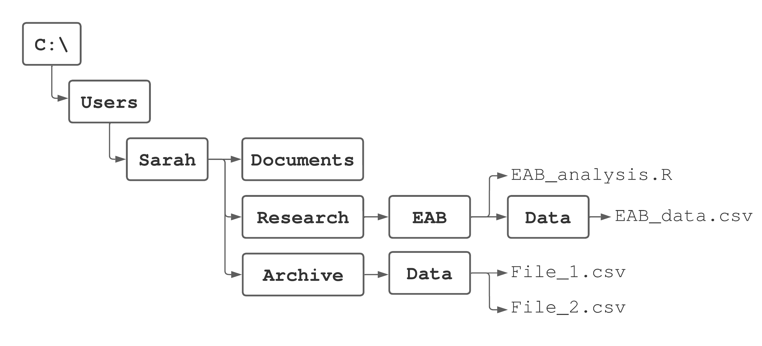
What is the root directory?

01:00

What is the root directory?

C:/

What is the home directory?

01:00

What is the home directory?

C:/Users/Sarah

How do we specify the absolute path to File_1.csv?

01:00

How do we specify the absolute path to File_1.csv?

C:/Users/Sarah/Archive/Data/File_1.csv

How do we specify the relative path to File_1.csv, if Sarah’s home directory is her working directory?

01:00

How do we specify the relative path to File_1.csv, if Sarah’s home directory is her working directory?

Archive/Data/File_1.csv

How do we specify the relative path to File_1.csv, if Sarah’s home directory is C:/Users/Sarah/Documents?

01:00

How do we specify the relative path to File_1.csv, if Sarah’s home directory is C:/Users/Sarah/Documents?

../Archive/Data/File_1.csv

What’s going on with those two dots? (../)

01:00

• Using .. in a file path means “go back a level”

• Example: Say I want to access a file on my desktop:

  • /home/grayson/Desktop/important_file.pdf

• But, my working directory is as follows:

  • /home/grayson/Documents

• Q: What is the relative path to the important file on my desktop?

• A: ../Desktop/important_file.pdf

Now consider a different computer

01:00

• We have an absolute path to lab_01.qmd:

  • /home/elliot/Documents/for128/lab_01.qmd

• Say Elliot is using the following working directory:

  • /home/elliot/research/spatio_temporal

• Q1: What operating system might Elliot be using?

• Q2: What is the relative path to lab_01.qmd?

• A1: macOS or Linux

• A2: ../../for128/lab_01.qmd

Reading and writing data

Reading data

In this course, we’ll focus on reading 2-dimensional data (things that look like spreadsheets) into R.

Reading data

Reading data

Reading data

R includes a variety of functions for reading data efficiently. One of the most common is read.csv().

Reading data

R includes a variety of functions for reading data efficiently. One of the most common is read.csv().

To read data, we first may want to check our working directory:

getwd()

[1] "/home/grayson/courses/FOR128/FOR128.github.io/slides"

Reading data

R includes a variety of functions for reading data efficiently. One of the most common is read.csv().

To read data, we first may want to check our working directory:

getwd()

[1] "/home/grayson/courses/FOR128/FOR128.github.io/slides"

Then we can find the datasets folder. I’ve kept mine with my labs:

list.files("../labs/")

 [1] "datasets"             "FEF_trees.csv"        "lab_01_solutions.pdf"
 [4] "lab_01_solutions.qmd" "lab_01.qmd"           "lab_02.qmd"          
 [7] "lab_03_example.R"     "lab_03.html"          "lab_03.qmd"          
[10] "lab_04.qmd"           "lab_05.qmd"           "lab_06.qmd"          

Reading data

R includes a variety of functions for reading data efficiently. One of the most common is read.csv().

To read data, we first may want to check our working directory:

getwd()

[1] "/home/grayson/courses/FOR128/FOR128.github.io/slides"

Then we can find the datasets folder. I’ve kept mine with my labs:

list.files("../labs/")

 [1] "datasets"             "FEF_trees.csv"        "lab_01_solutions.pdf"
 [4] "lab_01_solutions.qmd" "lab_01.qmd"           "lab_02.qmd"          
 [7] "lab_03_example.R"     "lab_03.html"          "lab_03.qmd"          
[10] "lab_04.qmd"           "lab_05.qmd"           "lab_06.qmd"          

Now, given our working directory and datasets location, we specify a relative path and load in the data:

fef <- read.csv(file = "../labs/datasets/FEF_trees.csv")

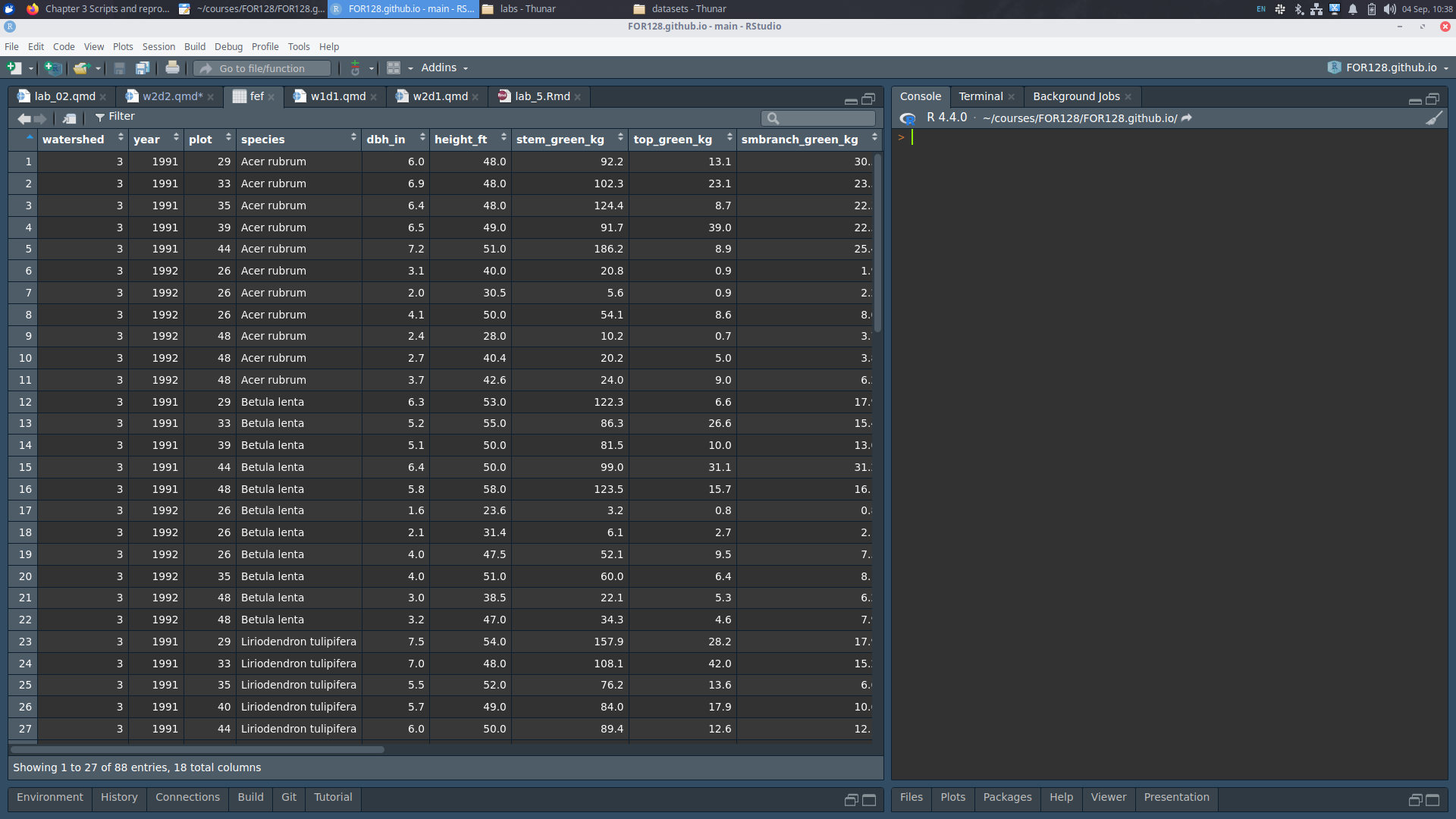
Reading data

We can take a look at our dataset in R:

dim(fef) # dimensions (rows columns) of fef

[1] 88 18

head(fef) # first few rows of fef

  watershed year plot     species dbh_in height_ft stem_green_kg top_green_kg
1         3 1991   29 Acer rubrum    6.0        48          92.2         13.1
2         3 1991   33 Acer rubrum    6.9        48         102.3         23.1
3         3 1991   35 Acer rubrum    6.4        48         124.4          8.7
4         3 1991   39 Acer rubrum    6.5        49          91.7         39.0
5         3 1991   44 Acer rubrum    7.2        51         186.2          8.9
6         3 1992   26 Acer rubrum    3.1        40          20.8          0.9
  smbranch_green_kg lgbranch_green_kg allwoody_green_kg leaves_green_kg
1              30.5              48.4             184.2            16.1
2              23.5              57.7             206.6            12.9
3              22.3              44.1             199.5            16.5
4              22.5              35.5             188.7            12.0
5              25.4              65.1             285.6            22.4
6               1.9               1.5              25.1             0.9
  stem_dry_kg top_dry_kg smbranch_dry_kg lgbranch_dry_kg allwoody_dry_kg
1        54.7        7.1            15.3            28.0           105.1
2        62.3       12.4            14.8            33.6           123.1
3        73.3        4.6            11.5            25.1           114.4
4        53.6       21.3            11.2            19.8           105.9
5       106.4        4.7            11.7            36.1           159.0
6        11.7        0.5             1.1             0.9            14.2
  leaves_dry_kg
1           6.1
2           4.6
3           6.1
4           4.2
5           7.9
6           0.3

Reading data

read.csv() reads comma separated value (csv) files, but R has the ability to read a massive variety of file types:

• read.table() allows you to read file types with different separators like tabs and spaces, rather than just commas.

Reading data

If we wanted to use read.table() to load in FEF_trees.csv, we would run the following code:

fef <- read.table(file = "../labs/datasets/FEF_trees.csv",
                  header = TRUE,
                  sep = ",")

Reading data

If we wanted to use read.table() to load in FEF_trees.csv, we would run the following code:

fef <- read.table(file = "../labs/datasets/FEF_trees.csv",
                  header = TRUE,
                  sep = ",")

Reading data

If we wanted to use read.table() to load in FEF_trees.csv, we would run the following code:

fef <- read.table(file = "../labs/datasets/FEF_trees.csv",
                  header = TRUE,
                  sep = ",")

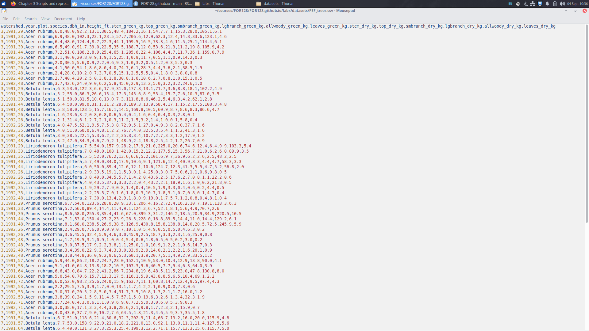
Reading data: tab separated

We also have the file FEF_trees.tsv, which looks a bit different than FEF_trees.csv.

FEF_trees.csv

FEF_trees.tsv

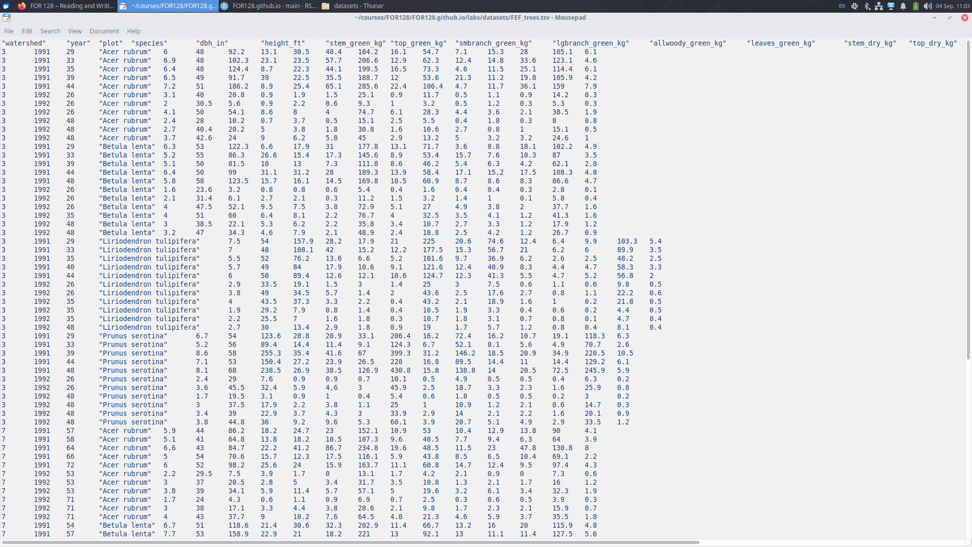
Reading FEF_trees.tsv into R

fef <- read.table(file = "../labs/datasets/FEF_trees.tsv",
                  header = TRUE,
                  sep = "\t")

Reading FEF_trees.tsv into R

fef <- read.table(file = "../labs/datasets/FEF_trees.tsv",
                  header = TRUE,
                  sep = "\t")

Writing data

• Similar to read.csv() and read.table(), R includes write.csv() and write.table() functions.

• These functions allow you to create (or “write”) your own files with an R object.

• Let’s take a look!

Writing data

First, we look at the files in my “labs” folder

list.files("../labs")

 [1] "datasets"             "FEF_trees.csv"        "lab_01_solutions.pdf"
 [4] "lab_01_solutions.qmd" "lab_01.qmd"           "lab_02.qmd"          
 [7] "lab_03_example.R"     "lab_03.html"          "lab_03.qmd"          
[10] "lab_04.qmd"           "lab_05.qmd"           "lab_06.qmd"          

Writing data

Next, we can write the fef object to a .csv file.

write.csv(x = fef,
          file = "../labs/my_fef.csv")

Writing data

Next, we can write the fef object to a .csv file.

write.csv(x = fef,
          file = "../labs/my_fef.csv")

Now, we can see that the file is written.

list.files("../labs")

 [1] "datasets"             "FEF_trees.csv"        "lab_01_solutions.pdf"
 [4] "lab_01_solutions.qmd" "lab_01.qmd"           "lab_02.qmd"          
 [7] "lab_03_example.R"     "lab_03.html"          "lab_03.qmd"          
[10] "lab_04.qmd"           "lab_05.qmd"           "lab_06.qmd"          
[13] "my_fef.csv"          

Next Week

• Andy will deliver lecture and lab through Tuesday 9/17.
• Main focuses: Chapter 4 (Data Structures).

See you upstairs in lab!