knitr::include_graphics("NETN_Parks.png")
Nicole Bommarito
Abigail Matson
Avrie Hoell
Kaily Hurt
Voka Schiller
December 9, 2024
In our project we chose to work with the Northeast Temperate Inventory & Monitoring Network (NETN),(2006-2004) data package from The National Park Data Base. Using this data, we aim to analyze the relationship between tree growth and the environment as well as the way trees can influence their environment. Specifically we investigate factors like the conditions of the forest floor and their relation to tree height classification, for both how fores
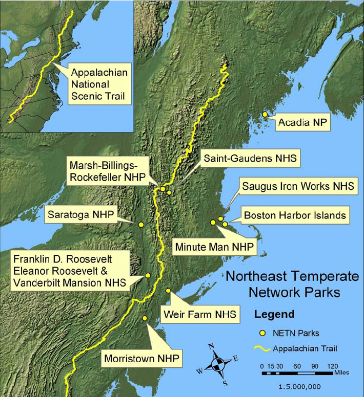
The NETN data set includes the 13 parks within the network which fall along the eastern coast of the united states, stretching from Maine to New Jersey. It monitors each plot once per year, stretching 18 years so far.
This CSV in the data set examines the Tree Foliage of plots within these parks
[1] 35511 30| Plot_Name | Network | ParkUnit | ParkSubUnit | PlotTypeCode | PlotCode | IsAbandoned | PanelCode | SampleDate | IsQAQC |
|---|---|---|---|---|---|---|---|---|---|
| SAGA-017 | NETN | SAGA | SAGA | VS | 17 | FALSE | 3 | 2012-06-14 | FALSE |
| ROVA-004 | NETN | ROVA | ROVA_HOFR_West | VS | 4 | FALSE | 2 | 2011-06-02 | FALSE |
| ACAD-057 | NETN | ACAD | ACAD_MDI | VS | 57 | FALSE | 2 | 2019-06-19 | FALSE |
| SARA-021 | NETN | SARA | SARA | VS | 21 | FALSE | 3 | 2008-06-02 | FALSE |
| MABI-023 | NETN | MABI | MABI | VS | 23 | FALSE | 3 | 2016-06-08 | FALSE |
| ACAD-034 | NETN | ACAD | ACAD_MDI | VS | 34 | FALSE | 1 | 2010-07-14 | FALSE |
This next CSV examines 5 different forest floor conditions within the parks as well as their health and height
[1] 10158 21| Plot_Name | Network | ParkUnit | ParkSubUnit | PlotTypeCode | PlotCode |
|---|---|---|---|---|---|
| ACAD-001 | NETN | ACAD | ACAD_Schoodic | VS | 1 |
| ACAD-001 | NETN | ACAD | ACAD_Schoodic | VS | 1 |
| ACAD-001 | NETN | ACAD | ACAD_Schoodic | VS | 1 |
| ACAD-001 | NETN | ACAD | ACAD_Schoodic | VS | 1 |
| ACAD-001 | NETN | ACAD | ACAD_Schoodic | VS | 1 |
| ACAD-001 | NETN | ACAD | ACAD_Schoodic | VS | 1 |
This CSV examines different individual trees, plots, and their height over the years
| Plot_Name | Network | ParkUnit | ParkSubUnit | PlotTypeCode | PlotCode | IsAbandoned | PanelCode | SampleDate | IsQAQC |
|---|---|---|---|---|---|---|---|---|---|
| ACAD-001 | NETN | ACAD | ACAD_Schoodic | VS | 1 | FALSE | 1 | 6/6/2006 | FALSE |
| ACAD-001 | NETN | ACAD | ACAD_Schoodic | VS | 1 | FALSE | 1 | 6/6/2006 | FALSE |
| ACAD-001 | NETN | ACAD | ACAD_Schoodic | VS | 1 | FALSE | 1 | 6/6/2006 | FALSE |
| ACAD-001 | NETN | ACAD | ACAD_Schoodic | VS | 1 | FALSE | 1 | 6/6/2006 | FALSE |
| ACAD-001 | NETN | ACAD | ACAD_Schoodic | VS | 1 | FALSE | 1 | 6/6/2006 | FALSE |
| ACAD-001 | NETN | ACAD | ACAD_Schoodic | VS | 1 | FALSE | 1 | 6/6/2006 | FALSE |
[1] 6876 21| Plot_Name | Network | ParkUnit | ParkSubUnit | PlotTypeCode | PlotCode | IsAbandoned | PanelCode | SampleDate | IsQAQC |
|---|---|---|---|---|---|---|---|---|---|
| ACAD-009 | NETN | ACAD | ACAD_MDI | VS | 9 | FALSE | 1 | 2006-06-14 | FALSE |
| ACAD-009 | NETN | ACAD | ACAD_MDI | VS | 9 | FALSE | 1 | 2010-07-13 | FALSE |
| ACAD-139 | NETN | ACAD | ACAD_MDI | VS | 139 | FALSE | 4 | 2009-07-08 | FALSE |
| ROVA-024 | NETN | ROVA | ROVA_VAMA | VS | 24 | FALSE | 4 | 2009-06-04 | FALSE |
| MABI-006 | NETN | MABI | MABI | VS | 6 | FALSE | 1 | 2006-07-26 | FALSE |
| MABI-007 | NETN | MABI | MABI | VS | 7 | FALSE | 1 | 2010-06-10 | FALSE |
The 4th CSV measures individual trees and what conditions they classify under
tree_conditions <- read_csv("TreesConditions_NETN.csv", show_col_types = FALSE)
dim(tree_conditions)
[1] 37464 55| Plot_Name | Network | ParkUnit | ParkSubUnit | PlotTypeCode | PlotCode | IsAbandoned | PanelCode | SampleDate | IsQAQC |
|---|---|---|---|---|---|---|---|---|---|
| ACAD-001 | NETN | ACAD | ACAD_Schoodic | VS | 1 | FALSE | 1 | 2006-06-06 | FALSE |
| ACAD-001 | NETN | ACAD | ACAD_Schoodic | VS | 1 | FALSE | 1 | 2006-06-06 | FALSE |
| ACAD-001 | NETN | ACAD | ACAD_Schoodic | VS | 1 | FALSE | 1 | 2006-06-06 | FALSE |
| ACAD-001 | NETN | ACAD | ACAD_Schoodic | VS | 1 | FALSE | 1 | 2006-06-06 | FALSE |
| ACAD-001 | NETN | ACAD | ACAD_Schoodic | VS | 1 | FALSE | 1 | 2006-06-06 | FALSE |
| ACAD-001 | NETN | ACAD | ACAD_Schoodic | VS | 1 | FALSE | 1 | 2006-06-06 | FALSE |
Finally, the last data set examines the plant cover within the plots ( notably it can not individual trees)
| Plot_Name | Network | ParkUnit | ParkSubUnit | PlotTypeCode | PlotCode | IsAbandoned | PanelCode | SampleDate | IsQAQC |
|---|---|---|---|---|---|---|---|---|---|
| ACAD-001 | NETN | ACAD | ACAD_Schoodic | VS | 1 | FALSE | 1 | 2006-06-06 | FALSE |
| ACAD-001 | NETN | ACAD | ACAD_Schoodic | VS | 1 | FALSE | 1 | 2006-06-06 | FALSE |
| ACAD-001 | NETN | ACAD | ACAD_Schoodic | VS | 1 | FALSE | 1 | 2006-06-06 | FALSE |
| ACAD-001 | NETN | ACAD | ACAD_Schoodic | VS | 1 | FALSE | 1 | 2010-07-27 | FALSE |
| ACAD-001 | NETN | ACAD | ACAD_Schoodic | VS | 1 | FALSE | 1 | 2010-07-27 | FALSE |
| ACAD-001 | NETN | ACAD | ACAD_Schoodic | VS | 1 | FALSE | 1 | 2010-07-27 | FALSE |
This data set has a lot of columns, to make it easier to work with we are going to remove columns not relevant to what we are trying to investigate.
We are also going to be pivoting our forest floor data set to tidy it up
Now that our data is cleaner, we need to combine the CSV datasets into one dataset we can work from
forest_floor and plant_cover join
forest_floor <- forest_floor %>%
group_by(ForestFloorLabel) %>%
mutate(row = row_number()) %>%
tidyr::pivot_wider(names_from = ForestFloorLabel, values_from = CoverClassCode)

plant_cover <- plant_cover %>%
group_by(StrataLabel) %>%
mutate(row = row_number()) %>%
tidyr::pivot_wider(names_from = StrataLabel, values_from = CoverClassCode)

combined_forest_plant <- left_join(forest_floor, plant_cover, by = c("row", "Network", "ParkUnit", "ParkSubUnit", "PanelCode","PlotID")) %>%
select(-Plot_Name.y, -SampleYear.y)combined_forest_plant_long <- combined_forest_plant %>%
pivot_longer(cols = c("Bare Soil", "Rock", "Water", "Trampled", "Non-Vascular", "Lichen"),
names_to = "Condition_Type", values_to = "Condition_Value")
combined_forest_plant_long <- combined_forest_plant_long %>%
filter(!Condition_Value %in% c("NC", "PM", "0"))
P1<- ggplot(combined_forest_plant_long, aes(x = Condition_Type, fill = Condition_Value)) +
geom_bar(position = "dodge") +
labs(title = "Distribution of Condition Types Across Forest Floor Coverage",
x = "Condition Type", y = "Count") +
facet_wrap(~ParkUnit, scales = "free") +
theme_bw()ggsave("condition_types.png", plot = P1, width = 20, height = 15)
knitr::include_graphics("condition_types.png")
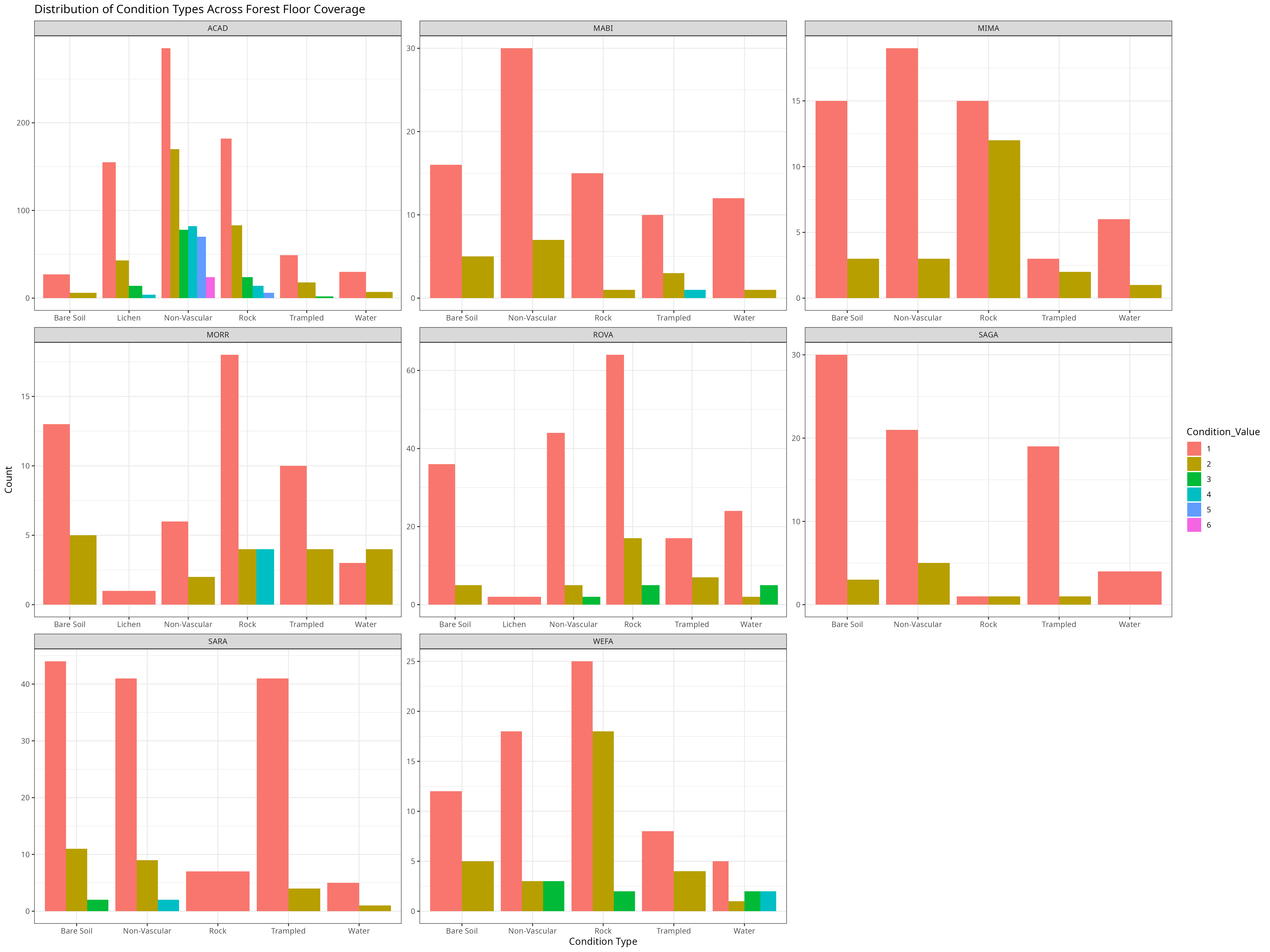
For this graph we filtered out conditions like 0, which indicated this condition type covered 0% of the forest floor and conditions like “permanently missing” or “not collected”. As we can see, the condition’s vary greatly across the parks. Many do not ever experience the “Lichen” condition which is a combination of fungus an algae. For most parks in this data set, conditions like “Non-vascular” or Rock tend to often cover at least a small percentage of the surface area of the plots within the park. These observations may in part be due to park size and number of trees ( as you can see the counts are much higher for Acadia (ACAD) than many of the other parks in the network). This insight into the forest floor compositions of the parks can help us identify which forest floor conditions are positively correlated with average tree height within the park over time.
combined_long_coverage <- combined_forest_plant %>%
  pivot_longer(cols = c("Ground", "Mid-understory", "High-understory"),
               names_to = "Condition_Type",
               values_to = "Vascular_Coverage_Rating")

P2 <- ggplot(combined_long_coverage, aes(x = Condition_Type, fill = as.factor(Vascular_Coverage_Rating))) +
  geom_bar(position = "stack") +
  facet_wrap(~ParkUnit,) +
  labs(title = "Count of Vascular Plant Coverage Ratings by Condition Type",
       x = "Condition Type", y = "Count of Coverage Rating") +
  scale_fill_brewer(palette = "Set3", name = "Vascular Coverage Rating (1-6)") +
theme_minimal() ggsave("vascular_coverage_plot.png", plot = P2, width = 20, height= 15)
knitr::include_graphics("vascular_coverage_plot.png")
The relationship between trees and the forest floor conditions can be bidirectional as well.
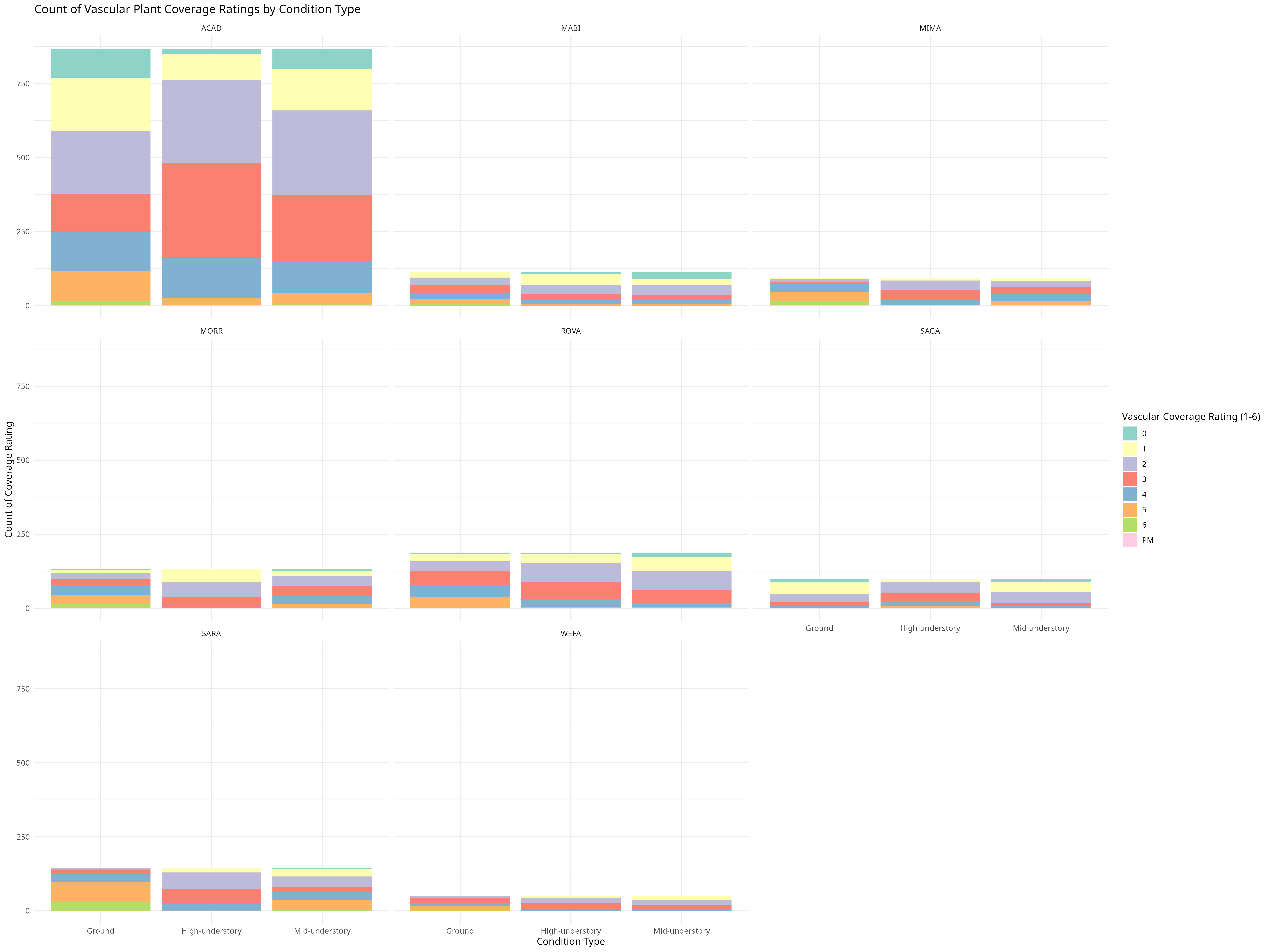
In this example the “Ground” condition represents trees that are less than 0.5 meters above ground, “Mid-understory” represents trees that have heights between 0.5 and 2 meters above ground, and “high understory” represents trees that are over 2 meters above ground. in height.
From what we can see in the graph, trees classified as”Ground” are the only trees with 95-100% vascular plant coverage on the forest floor, this phenomena is observed across parks,this could indicate that high vascular plant coverage is negatively correlated with tree growth but it is more likely this observation is due to the fact that these trees lack large amounts of canopy cover due to their short stature, allowing for needed sunlight to reach the vascular plants on the forest floor. Also likely explaining why the taller trees tend to have higher counts of lower vascular plant coverage. Though interestingly, plots rated with 0% vascular plant coverage could be found across a variety of conditions. For example trees in Acadia National Park (ACAD) that were classified as “Ground” show the highest rates of 0% with high-understory showing the lowest. This may tie back to Acadia’s larger variety in conditions as well as high percentage of non-vascular plant forest floor coverage compared to other parks.
Tree_heights_clean <- tree_heights %>%
  filter(!is.na(TagCode))

Tree_heights_clean <- Tree_heights_clean %>%
  select(-PanelCode,
         -IsAbandoned,
         -SampleDate,
         -IsQAQC,
         -contains("DPL"),
         -ExportDate)
avg_tree_heights <- Tree_heights_clean %>%
  group_by(ParkUnit, SampleYear) %>%
  summarise(Average_Height = mean(Height, na.rm = TRUE))
`summarise()` has grouped output by 'ParkUnit'. You can override using the
`.groups` argument.ggplot(avg_tree_heights, aes(x = SampleYear, y = Average_Height, color = ParkUnit, group = ParkUnit)) +
geom_line() +
geom_point() +
labs(title = "Average Tree Height by Park Over Time",
x = "Year",
y = "Average Tree Height (meters)") +
theme_bw()
# A tibble: 58 × 3
# Groups:   ParkUnit [8]
   ParkUnit SampleYear Average_Height
   <chr>         <dbl>          <dbl>
 1 ACAD           2011           14.4
 2 ACAD           2012           15.2
 3 ACAD           2013           13.4
 4 ACAD           2014           12.8
 5 ACAD           2015           13.1
 6 ACAD           2016           14.2
 7 ACAD           2017           13.7
 8 ACAD           2018           13.0
 9 ACAD           2019           13.5
10 ACAD           2021           14.0
# ℹ 48 more rows| SampleYear | Average_Height |
|---|---|
| ACAD | |
| 2011 | 14.44887 |
| 2012 | 15.18538 |
| 2013 | 13.36230 |
| 2014 | 12.78370 |
| 2015 | 13.10598 |
| 2016 | 14.15951 |
| 2017 | 13.72857 |
| 2018 | 12.98045 |
| 2019 | 13.51667 |
| 2021 | 13.99456 |
| 2022 | 13.37591 |
| 2023 | 13.45625 |
| 2024 | 14.31102 |
| MABI | |
| 2012 | 29.03333 |
| 2014 | 25.30149 |
| 2016 | 25.83922 |
| 2018 | 25.58438 |
| 2022 | 25.61698 |
| 2023 | 25.14545 |
| MIMA | |
| 2012 | 20.65938 |
| 2014 | 22.32632 |
| 2016 | 17.41277 |
| 2018 | 22.12000 |
| 2022 | 19.53750 |
| 2023 | 22.83929 |
| MORR | |
| 2011 | 30.55250 |
| 2013 | 28.77273 |
| 2015 | 25.51268 |
| 2017 | 28.09286 |
| 2019 | 27.67941 |
| 2022 | 27.47959 |
| 2024 | 27.74531 |
| ROVA | |
| 2011 | 24.81692 |
| 2013 | 23.14842 |
| 2015 | 22.50488 |
| 2017 | 23.78108 |
| 2019 | 23.10168 |
| 2022 | 22.11458 |
| 2024 | 24.11346 |
| SAGA | |
| 2012 | 26.67576 |
| 2014 | 26.19153 |
| 2016 | 24.36533 |
| 2018 | 25.44545 |
| 2022 | 23.27812 |
| 2023 | 24.63030 |
| SARA | |
| 2012 | 23.80976 |
| 2014 | 18.64789 |
| 2016 | 21.14571 |
| 2018 | 19.65571 |
| 2022 | 22.68406 |
| 2023 | 20.27639 |
| WEFA | |
| 2011 | 24.25333 |
| 2013 | 22.26923 |
| 2015 | 22.28667 |
| 2017 | 21.32143 |
| 2019 | 22.55172 |
| 2022 | 23.18571 |
| 2024 | 24.27632 |
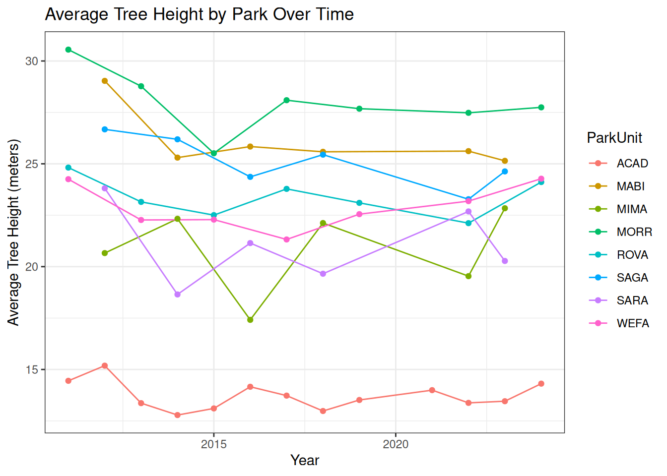
A lot of interesting conclusions can be drawn from this graphic and table
For example as you can see the “WEFA” (Weir Farm National Historical Park) park has significantly shorter trees than the other parks in the NETN network, Though this significant difference cannot be explained by tree height alone, when you look back to it’s forest floor data you notice high proportions of the forest floor conditions “Rock” and “Trampled” as well as “Bare Soil”, WEFA also has well as higher percentages of high vascular plant coverage. Similar trends can be seen for other low ranking parks like MIMA which has a forest floor predominantly consisting of rock.
Another interesting thing you can observe through this data is the dip in tree heights experienced across all parks in the network in the early 2010s. This points to some sort of event in the area that likely killed off some of the taller trees in the parks. It also indicates forest floor conditions as a relatively unimportant factor in accounting for a park’s average tree heights in the face of environmental events.
Fortunately, you can also observe consistent gains on the average tree heights across the parks indicating these trees are living longer and growing taller. However some parks like SARA (Saratoga National Historical Park) continue to suffer in terms of average tree height. Indicating once again, more park specific environmental factors outside of forest floor condition to be the root of their average tree height decline.
#Conclusions
Overall, in our analysis of the relation between parks, forest floor conditions, and tree height. We found forest floor conditions to exhibit a mild correlation with tree height. In our graphical observations parks with higher proportion of rock and bare soil were shown to have fewer trees as well as shorter trees. This lower average tree height indicates a large proportion of shorter trees and thus more vascular plant coverage. This was observed in many parks who tended to rank lower on average height across years, these parks had large proportions of high vascular plan coverage within their “Ground” trees category. However, when observing the trends over time it is clear that forest floor conditions are more influenced by tree heights than tree heights are influenced by the forest floor. Significant changes in tree heights were observed during specific time periods indicating a regional/ park specific event that likely killed older, taller trees. Showing that even in forests with great conditions for tree growth, catastrophic environmental events can set forest growth back more than anything.