Introduction

This is an example blog post about Western red cedar (Thuja plicata) trees in Portland, Oregon. I am using data from the pdxTrees R package. The pdxTrees R package has a nice hex sticker, which we can include in the blog post like this:

and if the image was on my computer rather than online, I could include it by using the same syntax with a relative path rather than website URL. Note the options I used to include this figure. “out-width” decides how wide the image should be, from 0% to 100%. “fig-align” allows you to align the image on the “left”, “center”, or “right”. “echo” either includes the code (echo: true) or does not include the code (echo: false) in the Rendered document. By default echo is true.

We’ll use a few packages for our analyses, namely the tidyverse, gt, and pdxTrees.

Code

library(tidyverse)
library(gt)
library(pdxTrees)

Note that we used the “code-fold” option here to fold the code used to load these libraries. We also set the “message” option to false in order to silence the message that the tidyverse prints upon loading.

Methods

Here we will discuss the two datasets we are using for this example project.

Park data

The parks data include measurements of every tree in every park in Portland, Oregon. We can load the data in as follows:

parks <- get_pdxTrees_parks()
dim(parks)

[1] 25534    34

By default, both the code and output is included.

The first few rows look like this:

head(parks)

# A tibble: 6 × 34
  Longitude Latitude UserID Genus       Family   DBH Inventory_Date      Species
      <dbl>    <dbl> <chr>  <chr>       <chr>  <dbl> <dttm>              <chr>  
1     -123.     45.6 1      Pseudotsuga Pinac…  37.4 2017-05-09 00:00:00 PSME   
2     -123.     45.6 2      Pseudotsuga Pinac…  32.5 2017-05-09 00:00:00 PSME   
3     -123.     45.6 3      Crataegus   Rosac…   9.7 2017-05-09 00:00:00 CRLA   
4     -123.     45.6 4      Quercus     Fagac…  10.3 2017-05-09 00:00:00 QURU   
5     -123.     45.6 5      Pseudotsuga Pinac…  33.2 2017-05-09 00:00:00 PSME   
6     -123.     45.6 6      Pseudotsuga Pinac…  32.1 2017-05-09 00:00:00 PSME   
# ℹ 26 more variables: Common_Name <chr>, Condition <chr>, Tree_Height <dbl>,
#   Crown_Width_NS <dbl>, Crown_Width_EW <dbl>, Crown_Base_Height <dbl>,
#   Collected_By <chr>, Park <chr>, Scientific_Name <chr>,
#   Functional_Type <chr>, Mature_Size <fct>, Native <chr>, Edible <chr>,
#   Nuisance <chr>, Structural_Value <dbl>, Carbon_Storage_lb <dbl>,
#   Carbon_Storage_value <dbl>, Carbon_Sequestration_lb <dbl>,
#   Carbon_Sequestration_value <dbl>, Stormwater_ft <dbl>, …

If we wanted to display the data in a more elegant way, we could use the gt package:

head(parks) %>% select(1:6) %>% gt()

Longitude	Latitude	UserID	Genus	Family	DBH
-122.6936	45.57491	1	Pseudotsuga	Pinaceae	37.4
-122.6938	45.57489	2	Pseudotsuga	Pinaceae	32.5
-122.6942	45.57493	3	Crataegus	Rosaceae	9.7
-122.6939	45.57490	4	Quercus	Fagaceae	10.3
-122.6940	45.57491	5	Pseudotsuga	Pinaceae	33.2
-122.6943	45.57489	6	Pseudotsuga	Pinaceae	32.1

We need to filter for only Western red cedars! So let’s do that:

Code

parks <- parks %>%
  filter(Species == "THPL")

In this case, we set the “code-fold” option to show rather than true or false, the show option allows the user to fold the code, but starts it as unfolded code.

Street data

We can also load in the streets dataset and include the code that was used to do that:

streets <- get_pdxTrees_streets() %>%
  filter(Species == "THPL")

Results

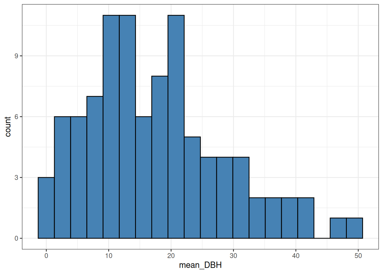
We can include plots and tables…

Code

parks %>%
  group_by(Park) %>%
  summarize(mean_DBH = mean(DBH)) %>%
  ggplot() +
  geom_histogram(aes(x = mean_DBH), 
                 color = "black", 
                 fill = "steelblue",
                 bins = 20) +
  theme_bw()

Code

parks %>%
  group_by(Park) %>%
  summarize(mean_DBH = mean(DBH),
            num_trees = n()) %>%
  slice_max(mean_DBH, n = 10) %>%
  gt()

Park	mean_DBH	num_trees
Thompson Park	50.00000	1
Joseph Wood Hill Park	47.80000	2
Johnson Creek Park	41.60000	2
Clinton Park	40.80000	1
Trenton Park	39.62000	5
Johnswood Property	38.76667	3
Gabriel Park	36.60000	23
Argay Park	36.44538	13
April Hill Park	34.25000	4
Kenton Park	32.64000	10

You can use the pipe to put a tibble right into a gt table

Conclusions

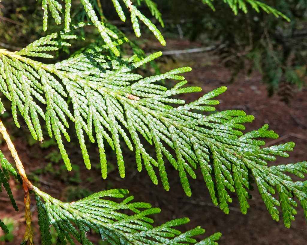
There are lots of beautiful Western red cedars in Portland! If I wanted to include a figure on my computer, I could do so like this:

knitr::include_graphics("wrc.jpeg")

Most of the time I would set echo: false for including an image, but I left it as true (the default) to show this example.